Revenue Forecast with ARIMA 2023.

Given the hospital revenue data from the last two years, how well can we forecast the revenue for an additional 30 days? One goal in this analysis is to use timeseries modeling to identify any patterns of prediction. One assumption of timeseries is stationarity, a constant mean and variance over time. If the variance and mean are constant, then the timeseries will exhibit no trends and the error term will be consistent. Meaning that the distribution shape will remain bell-shaped; Not right or left skewed, shrinking or expanding.  The error in the timeseries should be evenly distributed and the error is assumed to be uncorrelated (nist.gov). The residuals are not autocorrelated and no outliers should be in the data (Statistics Solutions, 2021). An ARIMA model requires 3 input variables to operate: P, D, Q. To get P, D, Q the data must be normalized for inspection. That means the data will be Lean Six-Sigma to extract the correct variable numbers.  

Below is a line graph visualizing the Times series of hospital revenue over the last two years and starting with an arbitrary date of “2011 -01-01”. The Graph shows the obvious trend in the data; The first visual indicator that there is stationarity.

Below is the code to format the date-time appropriately to an ARIMA model.

The Augmented Dickey-Fuller test is used to assess the stationarity of the data. If the critical values are less than the test statistic, then we have stationarity. When inspecting the absolute values of the ADF test statistic (2.21) and critical values at all percentiles are slightly higher. Slight seasonality because the Number of lags is 1 (variable ‘D’ for ARIMA) amongst 720 different observations.  

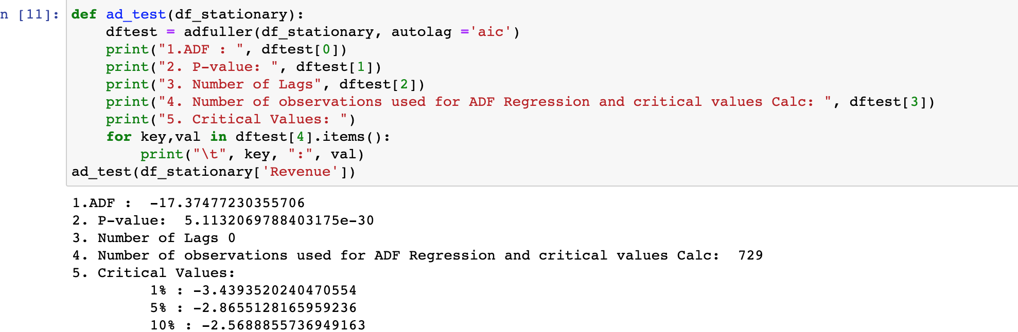
Stationarity was evoked after running differencing via .diff() method and retested via .adfuller(). Below is a photo of the retest, in which the ADF test statistic is higher than the critical values, therefore the data is stationary; Additional indication is the number of lags, 0.

The steps to prepare this dataset for analysis where as follows:

1.     Import the dataset as a .csv.

2.    Check for missing values with the isnull().any() method (there were no null values).

3.    Inspect the data size and output with the shape() and head() functions.

4.    Create a visualization of the data for any gaps or trends.

5.    Test for Seasonality via the adfuller().

6.    Differenced the data using the diff() method.

7.     Split the data into training and testing sets using the last 30 residuals (last 30 days) as a test set; Using 659 training points.

The first visualization shows the upward trend of the hospital revenue over time.

Below is a graph showing the lack of a seasonality as the all the residuals stay within less than 2 deviations from the mean indexed at 0.0.

Further inspection for seasonality with measures of central tendency in the time series when visualized with an autocorrelation_plot(); The result is a tight variance in the residuals and appears to tighten around 0.0. The following visualizations also indicate that there is no clear repeatable cycle.

Below is a visualization of Spectral Density, representing the lack of a periodicity and normalized data.

Moreover, exhibiting the same trend in the Autocorrelation and Partial Autocorrelation.

When fleshing out the data further with the seasonal_decompose()  on a monthly scale, only normalized data is evident. The below picture shows the scales of Revenue, Trend, Seasonality, and Residuals.

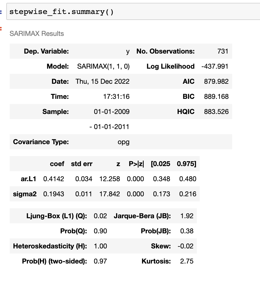
After passing the (non-differenced) data into an auto_arima() the best combination of P,D,Q for the model is (1,1,0), with the lowest AIC score. Since P and Q are cointegrated variables, only D, needs to be reconfirmed with the ADFuller test (Data Camp 2022).

Below is the visualized forecast from a derived ARIMA model when compared with the test data:

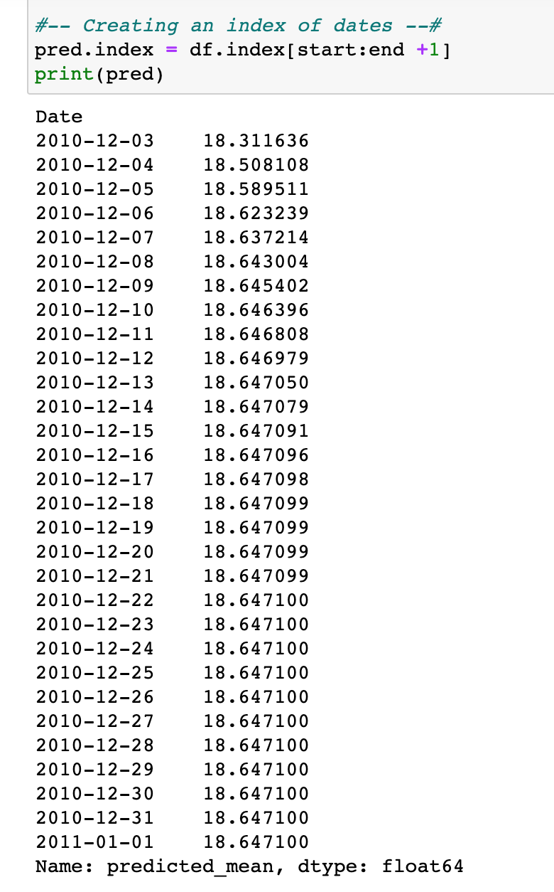
Below is the forecasted Hospital Revenue in for the next 30 days, an appropriate forecast window considering the small dataset of only 2 years.

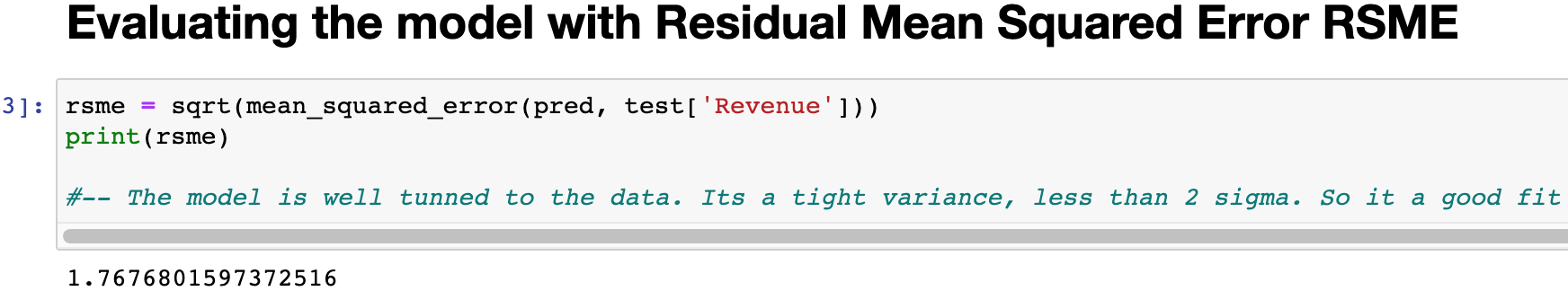
A Residual Mean Square Error of 1.76 indicates a very tight-fitting model to the dataset and correlates with the less than 2 Sigma deviance. Given that, the below predictions are reliable at a 98% confidence.

A recommended course of action would be to compile and compare more years of data to create a model that can forecast further into the future.

For more Data Science studies on Hospital Data check out Random Forest KNN Logistic Regression Tableau for Readmission prediction Market Basket Analysis for Prescription Data

Work Cited

Cointegration models: Python. campus.datacamp.com. (n.d.). Retrieved December 18, 2022, from Link

Stationarity Assumptions. 6.4.4.2. stationarity. (n.d.). Retrieved December 18, 2022, from Link

Time series analysis - understand terms and concepts. Statistics Solutions. (2021, September 16). Retrieved December 18, Link