A.I. and Natural Language Processing

Given the movie review dataset, what effect will Natural Language Processing have to predict the sentiment of future movie reviews? The following analysis can be converted into a very practical real-world tool. For example, reducing a YouTube video comments to a positive or negative can give a strong idea of the content of the video, without reading comments. Very practical if you are a media company that creates many videos with thousands of comments. Using the NLP and imdb movie reviews we can see how well a model can predict the sentiment of an individual review as positive or negative (that’s two categories of sentiment). A Recurrent Neural Network (RNN) is the type of Neural Network used because they can process temporal information, such as words and word-patterns.

Vocabulary size is the number of countable meaningful unique words, after you have removed the stop words. The vocabulary size of the dataset is 2,530 unique words. The proposed word embedding length is the longest review sentence length consisting of 677 characters after being parsed and processed. The goals of the Tokenization process is the accountability with labeled data, by taking individual words in a vector space and assigning them a number. When the data is labeled (semi- Supervised Learning) aka “word index”; A RNN model can then make inference (Unsupervised Learning) as to what the next word in a sentence might be when sequenced with other words and padded. One goal is to eliminate abnormal characters, standardizing, and formatting text. With that accomplished, synonymous word-phrases can be paired and analyzed.  Another goal is to ensure that padding preserves the shape of the biggest tensor’s dimension.

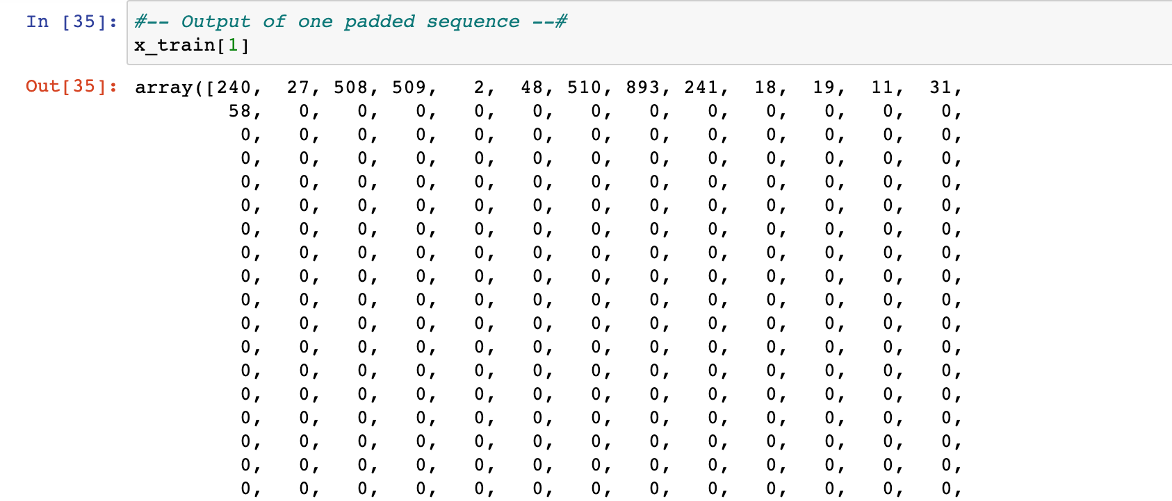
The process of the padding is to ensure that the longest sentence vector will be viewed in the first layer of the matrix. Accomplished with the tokenizer() from the Keras library. The tokenizer can be used for character / word parsing and labeling.  In this case, the padding will be “Post”; All text will be aligned to the left of the matrix and padded with zeros from the end of the sentence array to the right end of the array. The longest sentences will require little to no padding, while the rest of the sentence arrays will be aligned and padded. Padding causes each sentence to have the same number of tokens, so all sentences (all the same size) in a list can fit in the initial matrix layer; Therefore, if the longest sentence (array) isn’t the baseline, then statistically, many sentences may be excluded from the model.

First was to read the data from a .csv file into Pandas DataFrame and re-label the columns. Then used the dropna() function to get rid of missing values. Next, a hasty exploration with a bar chart to get a rough idea of the overall sentiment of that movie. Second, a for-loop was created that eliminates unusual characters and emojis using the ‘re’ (Regular Expression) method. Then the text is converted to lower case using the lower() function and the individual review-words / characters are parsed using the nltk.word_tokenize() function. A final nested for-loop is employed with a variable of common “stop_words” of the English language to filter the now tokenized text in the list. The individually labeled words are then appended to a list with a space separating them. Further data exploration, with for-loop that yields the minimum, medium, and maximum sentence length (vector array of words). From here, the list containing the word vector arrays are converted into a two-dimensional NumPy array.

Next, the data is split into training and testing sets with train_test_split(), which outputs a tuple of four variables label X_train, X_test, y_train, y_test. Then applying a tokenizer using the fit_on_texts() method to the training sets; Which creates a body of words to reference based on the review words. Directly after, the two ‘X’ variables (training sets) are transformed into sequences of commonly occurring words and given numeric labels; Accomplished with the text_to_sequences() function. Finally, the sequences are padded with the pad_sequences() function which covers the processed described earlier.

The model architecture is as follows: (1) embedding layer, (1) LSTM layer, (1) Dense layer, and (1) dropout layer. The activation function is “Sigmoid” because of the binary outcome will result in a Sigmoidal distribution shape. Embedding Layer: groups the word_index in into individual vectors, then attempts to infer the meanings and group those words with synonyms.

An LSTM layer was used because according to Kaggle.com, “LSTM can decide to keep or throw away data by considering the current input, previous output, and previous memory.” (2020). LSTM is good for cerebral processing and like the human brain, can forget useless information, retain old information, and make inference on new information. LSTM is best for categorical prediction, but it can be powerful for long-term binary predictions (which correspond to the research question). The final Dense layer is called as the predictive layer, activating by the Sigmiod and yeilding one output shape (0 or 1). The model is also yeilding 0 non-trainable parameters.

The below photo shows how the model loss started at 0.694 with an accuracy of 0.4833 after the first Epoch. The second Epoch yielded a slightly lower loss of 0.6925 and increase in accuracy to 0.4833; Peaking on the 3rd Epoch to an accuracy 0.5201 and troughing model loss at 0.6926. Then Epochs 4 and 5 produced worse metrics. Notice how the accuracy did not improve from a previous checkpoint test of 53%.

If the model doesn’t increase in accuracy after a certain number of iterations, then the stopping- function will cease; Early stopping saves computation time and ensures that the model isn’t overfit. In this case, after repeated tinkering with layers and dropout rates the model stopped improving and ceased after about 3 Epoch. However, to get more data for visualization, the number of epochs was set to 5 when fitting the model to the training data. Using the evaluation() metric, the accuracy yielded was 51.8%. The loss was near 70%, a very high cost for training the data. If there is no stopping criteria, then the model would be a runaway-loop as it continues to activate and train a neural network; The starting point of 5 Epochs was used as a small computational bracket to experiment with the model. If the model performance peaked at 5 Epochs then more Epochs would be added until the most optimal model is reached. The  Stopping Criteria saves processing power and time.

The model is trained only to that specific movie dataset, therefore is underfit to that training data. When evaluating the Confusion Matrix, the True Positive (TP) is 61, False Negative (FN) is 12, False Positive (FP) is 62, and True Negative (TN) is 15. The formula for Model Accuracy with a Confusion Matrix is (TP + TN) / (TP + TN + FP +FN); Which transcribes to (61 +15) / (61 + 15 +62 +12) = 50.6 % accuracy. According to numpyninja.com, the main objective of the model is attempt to replicate the human brain and its network of neurons to learn by automatically modifying itself (Kapoor, 2020).  In this case, the model is no better than a coin flip. A recommended course of action is to compile more review texts to increase the vocabulary size of the data-set and may increase accuracy. Another course of action is re-compiling the Tensorflow flags to take the governor off the optimization process off this Mac’s GPU or running the Python code on the new Macintosh M1.

Work Cited:

“Adam.” Adam - Cornell University Computational Optimization Open Textbook - Optimization Wiki, https://optimization.cbe.cornell.edu/index.php?title=Adam.

Kapoor, N. (2020, October 30). Neural network and its functionality. Numpy Ninja. Retrieved January 5, 2023, from https://www.numpyninja.com/post/neural-network-and-its-functionality

pawan2905. “IMDB Sentiment Analysis.” Kaggle, Kaggle, 10 May 2021, https://www.kaggle.com/code/pawan2905/imdb-sentiment-analysis.