

How to Detect Malware with Random Forest?

Abstract:
Bottom Line Up Front: Detect Malware with 95% accuracy using a Random Forest.
This paper investigates the development of a descriptive and predictive Random Forest model for detecting malware attempting to access ports in cybersecurity data. The research question addressed is whether such a model can be constructed effectively. The null hypothesis posits that the Random Forest model lacks significant classification power and performs no better than random guessing, while the alternative hypothesis asserts the opposite. Leveraging an open-source dataset of Counter Threat Unit (CTU) conn.log scans from Kaggle, this study focuses on a subset of variables to predict malware activity. By employing Random Forest regression tests, the research aims to enhance cyber defense strategies, optimizing investment in port security measures. Methodologically, the study employs various data analytics tools and techniques, including KDE plots, Pearson's correlation matrix, and Random Forest regression tests implemented in Python using scikit-learn. The project outcomes include the development of a descriptive statistical model, exploratory visualizations, and a better understanding of malicious request patterns. Findings indicate that the Random Forest model exhibits significant classification power, outperforming random guessing in detecting malware, as evidenced by high accuracy scores and performance metrics. These results underscore the potential of Random Forest algorithms in cybersecurity applications, paving the way for further research and exploration in this domain.
Research Question:
Can a Random Forest predictive model be developed from the data?
Null Hypothesis (H0): The Random Forest model has no significant classification power, and its performance is not better than random guessing.
Alternative Hypothesis (H1): The Random Forest model has significant classification power, and its performance is better than random guessing.
Context:
The contribution of this study to the field of Data Analytics and Cyber Security is to create a Random Forest Regression test to predict malware attempting to access ports. With this information a cyber security company can maximize the investment put into port security. An article titled, Random Forest Based Intrusion Detection Model, showcases a study using Random Forest to classify of ‘Label’, using similar variables of: ‘port_scan’, ‘heartbeart’, and ’DDoS’ (Chen Yu Zhu, 2024). They found that these variables are key factors in overall categorical accuracy. This research is one part of an overall big data study to create predictive models for all Security Information Emergency Management (SIEM) logs.
A Random Forest algorithm is an ensemble learning classification method which combines bagging and the random subspace algorithm. It tends to be a very high performing machine learning model very fast training speed and strong generalization ability. An ensemble method it can effectively prevent the overfitting problem by resampling via bootstrap the training data for each decision tree. After that the final prediction result is obtained and based on a voting algorithm by aggregating the prediction of different decision trees in the model. Additionally on ensemble methods can handle dirty data or data with missing values (scikitlearn, 2020).

Data:
An opensource dataset of Counter Threat Unit (CTU) conn.log scans of malware detection on network traffic data. Conn.logs. A Kaggle dataset from www.kaggle.com. Kaggle is the opensource repository / organization that hosts the datasets. Associated with the data on Kaggle, is a detailed break-down of all the variables from the data aggregating source, Stratosphereips.org. Stratosphereips.org has numerous terabytes of cyber security scans of all types. The dataset on Kaggle contains 10 datasets of 1 million rows each (total 10 million). For this analysis the dataset is limited to only the first 1 million rows to examine model generalization. The dataset has multiple columns for possible exploration. Delimitations for this analysis, of the original 23 columns only 13 will be considered in the initial exploration; Lastly, only 4 columns of the dataset will be used as they factor with no high multi-collinearity and 3 variables are germane to the target variable ‘label’: 'orig_ip_bytes', 'history', and 'id.orig_p'.
The datasets can be accessed at one of the two following links:
https://www.kaggle.com/datasets/datasnaek/youtube-new?select=USvideos.csv
Available to the public via Kaggle.com, meaning that the dataset may be limiting in accuracy and completeness. To get the unabridged copy, check out this link here:

Below are the variables that will factor into the prediction:
Data Gathering:
Plan and direct data gathering to opensource repositories (Google). Looking for keywords such as “cyber security”, “malware”, “datasets”, “+ .csv”. Next, selecting the 1st to 3rd ranked piece of content (reachable csv file) and inspecting each csv file for quality such as “length” (at least 7k rows), data cleanliness, massive gaps in data, and enough relevant variables to create an ‘X’ and ‘Y’ axis. In Random Forest Regressor intends to predict a continuous variable; Therefore, the dependent variable must be a continuous (interval or ratio) level of measurement (IBM, 2021). Fortunately, all dependent variables are numeric. The dataset is .04% sparse and all missing or null columns will be dropped when cleaning the dataset.
Data Analytics Tools and Techniques: A KDE plot was used to visualize the distributions of each relevant variable. A Person’s Correlation Matrix will assess the strength between the independent variables to the target variable. All variables with high-multicollinearity will be removed prior to further exploration. Random Forest is germane to studying this data because it can make powerful predictions and classifications on non-parametric data. Additionally, the Random Forest test does not assume normality in the data (sklearn, 2019). Overall, this is an exploratory quantitative data analytic technique and a predictive statistic. The tools used will be Jupyter Notebook operating in Python code, running sklearn api as a reliable open-source statistical library. Due to the data size, a Pandas data frame will be called, same with Numpy; Seaborn and Matplotlib will be used for visualizations. Next, the data will be scaled and passed into two unsupervised Machine Learning models, Principal Component Analysis (PCA) and Kmeans. PCA will be used to reduce the dimensionality and find the optimal number of clusters for Kmeans. Random Forrest is germane to studying this data because it can make powerful predictions and classifications on non-parametric data. Additionally, the Random Forrest test does not assume normality in the data (sklearn, 2019). A Random Forest test will be the statistical test used with Sklearn’s RandomForestRegressor() function. A presentation layer will be used with the aid of Univariate and by Bivariate graphs.
Justification of Tools/Techniques:
Python will be used for this analysis because of Numpy and Pandas packages that can manipulate large datasets (IBM, 2021). The tools and techniques are common in industry practice and have consensus of trust. The technique is justified through the integer variables necessary to plot against a timeline. In so doing, may just reveal different modes of frequency distribution. Another reason why the Random Forest model is ideal is because the data is based off human hacking behavior, which is notoriously skewed. Because of the size of the dataset, pandas and Numpy will be called. Python is being selected over SAS because Python has better visualizations (Panday, 2022).
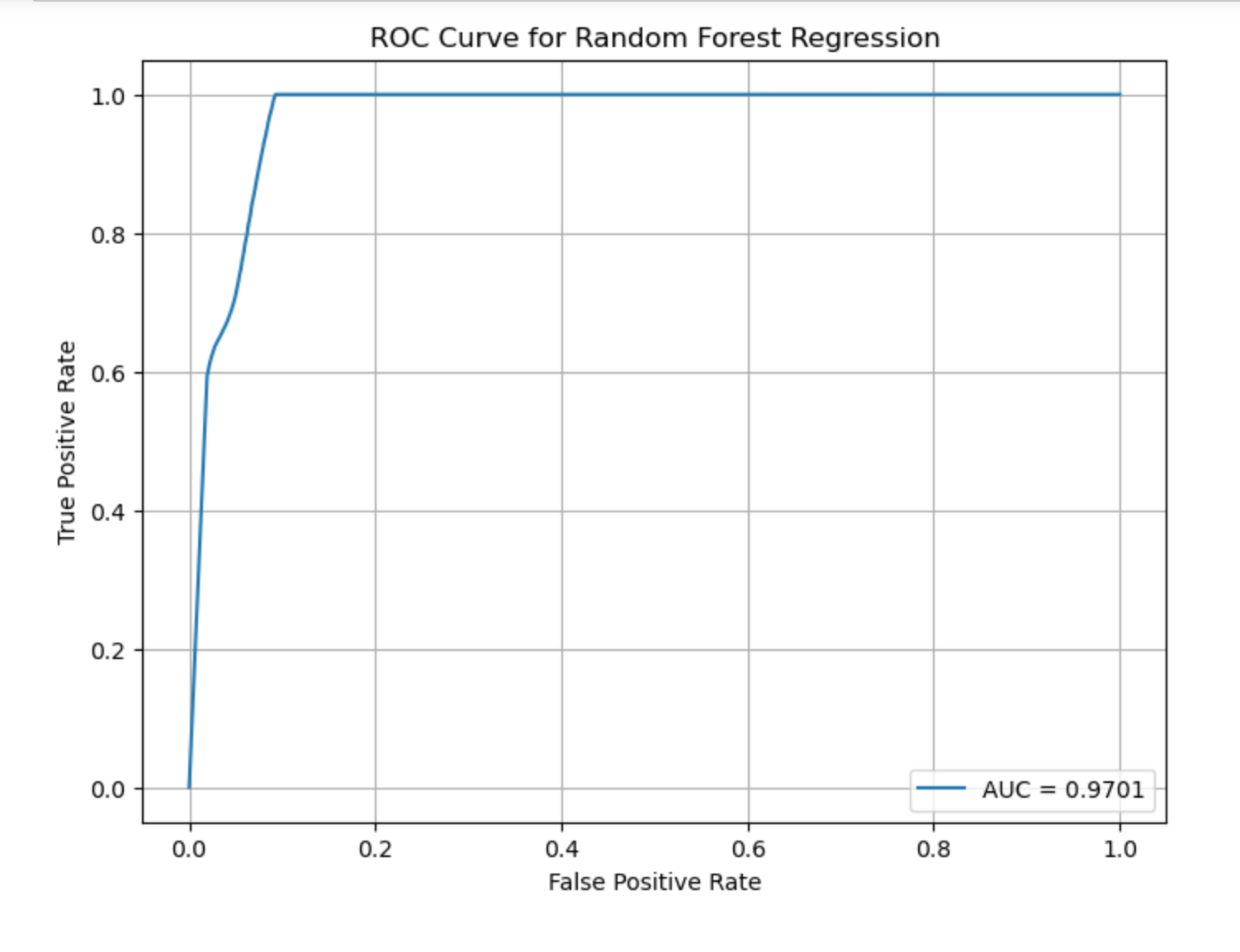
Project Outcomes: To find statistically significant differences, the proposed end state is a Random Forest Regressor descriptive statistical model that can classify malicious requests (Krieger, 2022). A visualization of the frequency distribution of the Random Forest, a Receiver Operator Characteristic ROC / Area Under the Curve visualization. A cleaned dataset of all the correctly labeled columns and rows, for replication. A better understanding of previously stated groups with exploratory graphs, giving support as to what latent variables are key to classification of malware. Lastly, a copy of the Jupyter NoteBook with the Python code will be available, along with a video presentation added by PowerPoint. According to the same study Random Forrest was instrumental in support for alternative hypothesis, against other categorical variables (Chen Yu Zhu, 2024).
Below is the python code with steps:
Follow along with the code on Github.


Step 2: Variable Exploration via Visualization
The first graph below is a correlation matrix aka (Pearson's Correlation matrix) or Heatmap. The correlation matrix visualizes the correlation coefficient, positive or negative, between the target variables ('label' in this case).
The correlation matrix is a Data Miner's gold pan; It picks out signal from the noise and exposes other hidden associations between variables. The trick is to remove all variables (and variable derivatives) that have a high association with "multi-collinearity' with the target variable; 'label' in this case.
Additionally, the associations between variables can sometimes be mathematically manipulated to create even better predictive variables, AKA "Feature Engineering".
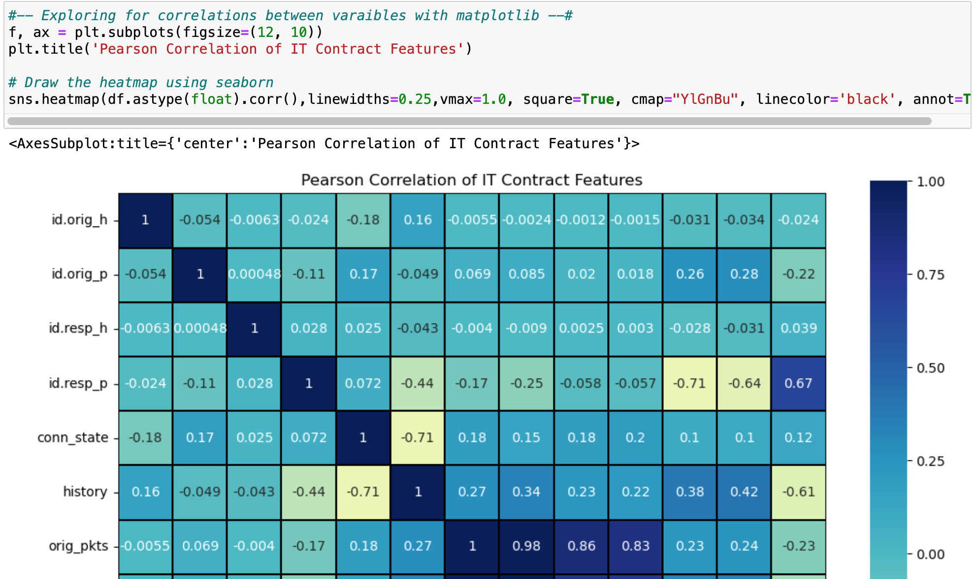

A correlation coefficient of 1 indicates a perfect positive linear relationship, -1 indicates a perfect negative linear relationship, and 0 indicates no linear relationship.
The above graph indicates multi-collinearity between the target variable "label" and the variables of 'proto_tcp' (92%) and 'id.resp_p' (-71%); They will be removed because they caused the model to overfit due to high- multicollinearity.
Thresholds and Cutoffs: Setting specific correlation coefficient thresholds for removal is not generally recommended as it can be overly simplistic and neglect other factors.
Now going into Univariate exploration with density.

Machine Learning is an Art: The process of model development and feature selection involves an iterative process of experimentation, evaluation, and refinement based on your specific data and problem. The art is to find the germane variables that will not cause the model to overfit and make more accurate predictions of unseen data.
The additional art is using only the variables necessary and no more; More variables will just add more noise to the model, reach a plateau of accuracy, then descend in accuracy, due to noise. Variable reduction increases computation.
Step 3: Univariate visualization exploration
An important step, the visuals generate the distribution shapes, indicating the parametric of non-parametric nature of the variables. If all variables look Gaussian ('bell-shaped' or not skewed) then a Shapiro-Wilk test will be used to test for "normality". Else, one or more of the variables is non-parametric, forcing the use of non-parametric machine learning models.


Step 4: Determine the parametric nature of the variables.
For the above univariate distribution plot or KDE visualizations, one or more of the variables is non-parametric in nature; Eliminating the need for the Shapiro-Wilk test and coercing the testing to non-parametric models only.
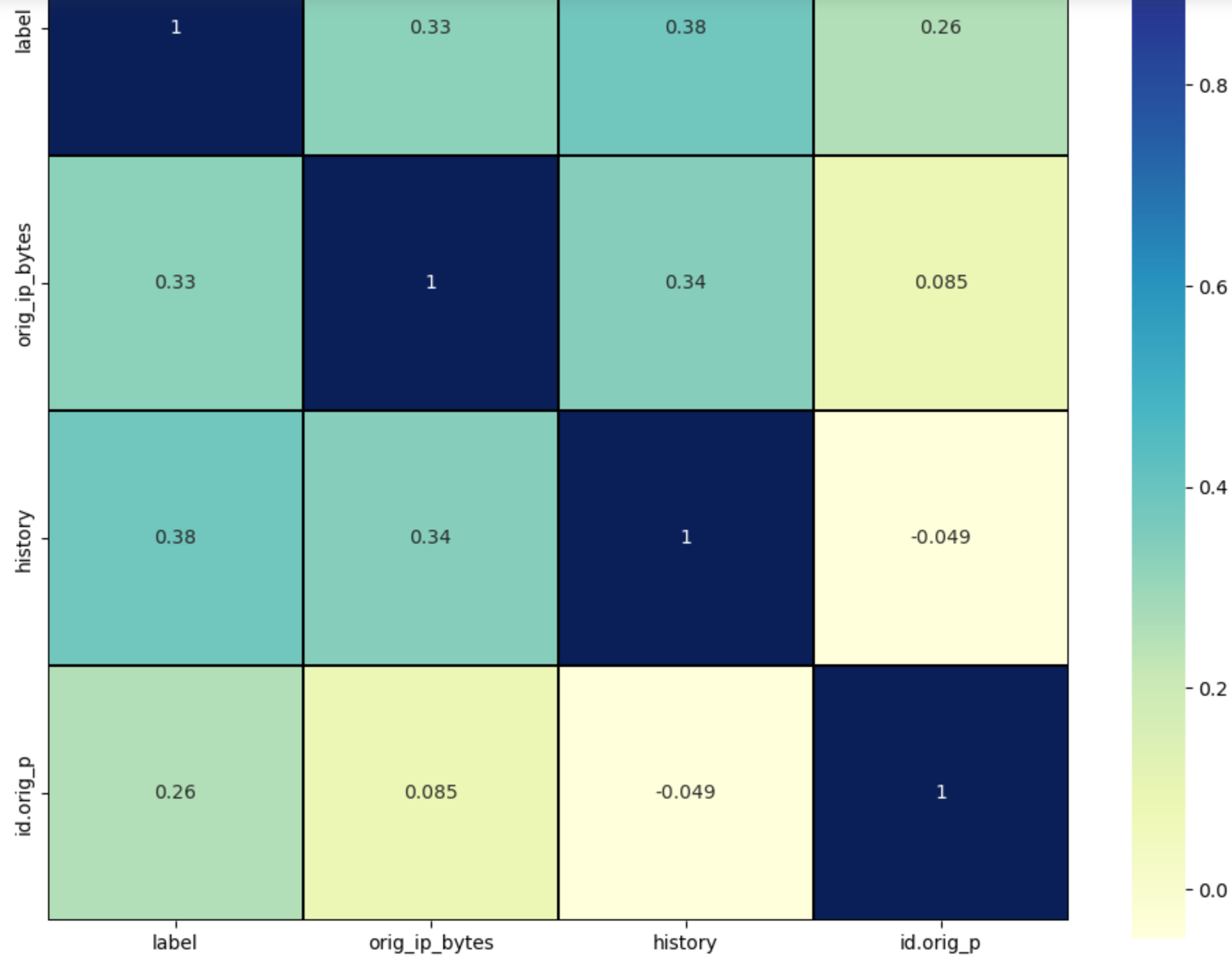
The below is a final verification via correlation matrix that all highly correlated variables have been removed.
Step 5: Exploratory Analysis via Unsupervised Machine Learning
The first Machine Learning model used is Principal Component Analysis (PCA). PCA helps determine the necessary number of variables for the model contingent upon the amount of variance contained in the variables. PCA is a dimensionality reduction technique that reduces variables to Principal Components. Reducing the variables to eigen vectors then eigen values.
Next, the Principal Components are explored via KMeans Cluster Analysis, another unsupervised machine learning technique.


According to the above graph, the Kaiser Criterion, and 'elbow method', the optimal number of variables / clusters is around 5.
Step 5.5: KMean Cluster Analysis, exploring the data in reduced dimensional space.
See like the machines, with KMeans.
Imagine you are in a spaceship, and you are approaching a galaxy from a distance and you ask your ship's auto-navigator to show you the entire galaxy as one grouping. The auto-navigator will move the spaceship to reorient in space, displaying to you the entire galaxy as one group. For each cluster number, the spaceship reorients in space / time, most effectively displaying to you the different star color groups in space-time.
Exploring Principal components in this space can reveal patterns that can be better understood or exploited by other machine learning models.

One cluster.

Two clusters.

Three clusters.

Four clusters.

The above visualizations do not look scattered or random, there appears to be structure in residuals, an indicator of predictability.


Below is a visualization of the Random Forest flowchart.


Step 8: Summarize the Findings
In final analysis, we reject the Null Hypothesis (H0) in favor of the Alternative Hypothesis (H1): The Random Forest model has significant predictive / classification power, and its performance is better than random guessing.
After cleaning and exploration, all variables with high-multicollinearity with the target variable were removed. The variables were displayed in density distribution charts and verified via the correlation matrix. Also, the distributions of one or more of the variables was non-parametric, justifying the use the ensemble methods.
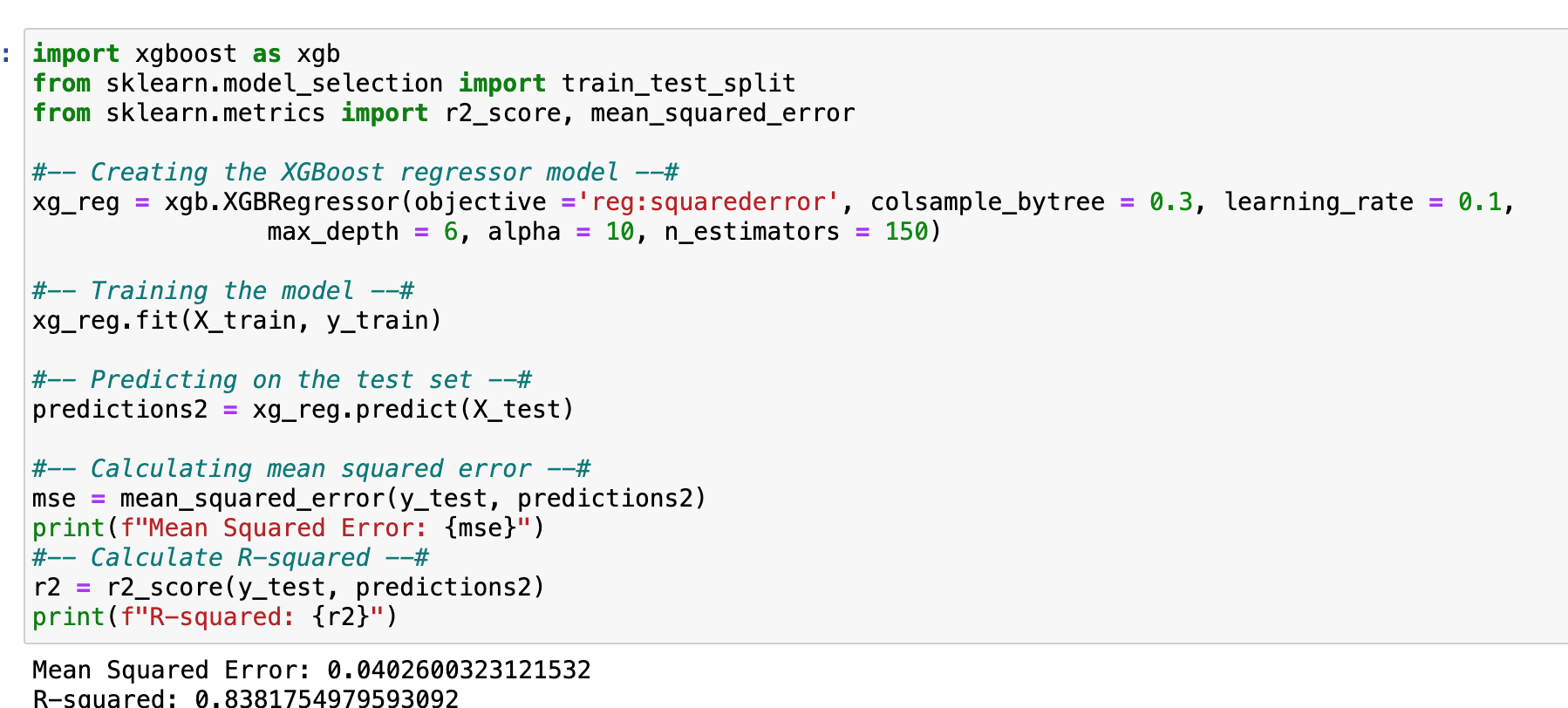
Both versions of Random Forest tested approximately the same. While the first model's Mean Squared Error: 0.043, R-squared: 0.826, Area Under the Curve (AUC)is 97%, total Accuracy: 0.953; Correspondingly, the Classification model yielded an R-squared (R2): 0.814, Mean Absolute Error (MAE): 0.046. In general, the R2 score should be as close to 1 as possible however, have an MEA close to '0', and an AUC of minimum 95%. The following precision scores indicate that the Random Forrest model should be able to generalize well on unseen data.
Different data sets should be compiled for additional testing. Moreover, other variables can be engineered and explored from the conn.log data. While the stated models outputted a high correctness, there are numerous non-parametric machine learning models that can be explored with the data.
This concludes the initial big data investigation for the conn.log in the scientific exploration Security Information Event Management (SIEM) logs.
Bottom Line: Detect Malware with 95% accuracy using a Random Forrest.
Work Cited
1.11. ensembles: Gradient boosting, random forests, bagging, voting, stacking. scikit. (n.d.). https://scikit-learn.org/stable/modules/ensemble.html
Conn.log| IP, TCP, UDP, ICMP connection details. (n.d.). https://www.icir.org/vern/cs261n-Sp20/slides/Protocols.pdf
Kreiger, J. (2021, September 10). Evaluating a random forest model. Medium. https://medium.com/analytics-vidhya/evaluating-a-random-forest-model-9d165595ad56
Pandey, Y. (2022, May 25). SAS vs python. LinkedIn. https://www.linkedin.com/pulse/sas-vs-python-yuvaraj-pandey/
Team, I. C. (2021, March 23). Python vs. R: What’s the difference? IBM Blog. https://www.ibm.com/cloud/blog/python-vs-r
