Abstract

Bottom Line Up Front: Between 0500 and 0700 Zulu time appears to be prime time for video engagement on YouTube.

A media company wants to explore the best time to upload videos to YouTube. The study takes a YouTube trending videos dataset for the United States and explores it. The dataset was extracted, cleaned, and statistically tested. The analysis compares the video engagement metrics of ‘likes’, ‘dislikes’, ‘views’, and ‘comment_count’. These different groups were tested for normality via Shapiro -Wilk test. The results of the Shapiro-Wilk test confirmed that the stated variables are non-parametric. Furthermore, a Kruskal-Wallis test was appropriate to investigate differences between two or more groups. Resulting, in two or more groups being different. During data exploration a metric Engagement Per View EPV, was created with all four non-parametric variables. The result was a parametric variable, that tested positive for being Gaussian in the Shapiro-Wilk test. The exploration yielded interesting insights; When plotted individually, the variable’s distributions skewed one direction, then when plotted against ‘upload_hour’, all skews changed directions (except ‘dislikes’). When plotted against ‘upload_hour’, EPV showcases a perfect bell-shape right along the 0500 to 0700 Zulu hour. Contrastingly, the highest frequency of video uploads is occurring during the 1600 Zulu hour.

Research Question:

Can a descriptive Kruskal-Wallis model be developed from the data?

Null Hypothesis H0:

There is no difference between the distributions of the scores of these four populations.

Alternative Hypothesis H1:

At least two of the four populations differ.

The contribution of this study to the field of Data Analytics and the MSDA program is to create a Kruskal-Wallis test to investigate prime upload hours on YouTube. With this information a media company can maximize the investment put into the video content. An article titled, Brand Engagement in Light of Post Content Type on the Facebook Platform in the Selected Industry, showcases a study using Kruskal-Wallis testing to explore engagement strength using the identical variables of ‘Likes’, ‘Views’, and ‘Comment Count’ (GATR, 2020). They found that these variables are key factors in overall content engagement and brand awareness. The Kruskal-Wallis H-test, tests the null hypothesis that the population median of all of the groups are equal. It is a non-parametric version of ANOVA (Scipy, 2020). Understanding these variables can help describe the relationship between the IV and DVs.

Data Collection

An opensource dataset of YouTube data containing the necessary variables about video uploads. A Kaggle dataset from www.kaggle.com. Kaggle is the opensource repository / organization that hosts the datasets. The dataset contains almost 40,950 rows (before any rows were removed) and 16 columns. The dataset is limited to only 7 months of YouTube’s trending videos; Uploaded from 2017 – 2018. The dataset has multiple columns for possible exploration. Different audiences watch shows at different time-zones all over the planet. Delimitations for this analysis, only 5 columns of the dataset will be used as they are factors of engagement: The ‘published_time’, ‘views’, ‘likes’, ‘dislikes’, and ‘comment_count’; The dataset is easy to work with because the columns with whole integer values. The ‘published_time’ is in 24hour timestamp indexed on Zulu time (located in England). The time will need to be separated from the date. Limitations are data size, and the type of variables contain. The delimitation of the study is that of the 16 columns only 5 will be used.

Available to the public via Kaggle.com, meaning that the dataset may be limiting in accuracy and completeness. The clickable link is located below:

https://www.kaggle.com/datasets/datasnaek/youtube-new?select=USvideos.csv

Below is a picture of the variables to be used along with the data type.

Data Gathering:

Planning and direction of data gathering was from opensource repositories (Google). Searching for keywords such as “YouTube”, “Videos”, “upload times”, “+ .csv”. Next, selecting the 1st to 3rd ranked piece of content and checking the availability (a reachable csv file). Each csv file was inspected for quality such as “length” (at least 7k rows), data cleanliness, massive gaps in data. Cross examined to ensure there was enough relevant variables to create an ‘X’ and ‘Y’ axis. Available to the public via Kaggle.com means that it may be limiting in accuracy and completeness. In Kruskal-Wallis, the dependent variable must be a continuous (interval or ratio) level of measurement (Statology, 2019). Fortunately, all dependent variables are continuous. The dataset is 1.4 % sparse and all missing or null columns will be dropped when cleaning the dataset. The ‘upload_time’ will be separated from the date in Microsoft Excel into a numerical category of twenty-four separate hour categories.

Data Extraction and Preparation:

A KDE plot is used to visualize the distribution and Shapiro-Wilk is used to test for normality. Kruskal-Wallis is germane to studying this data because it can compare distributions of non-parametric data. However, the Kruskal-Wallis test does not assume normality in the data (Statology, 2019). Overall, this is an exploratory quantitative data analytic technique and a descriptive statistic. The tools used will be Jupyter Notebook operating Python code, running statsmodel API as a reliable open-source statistical library. Due to the data size, a Pandas data frame will be called, same with Numpy and Seaborn will be used for visualizations. A Kruskal-Wallis test will be the statistical test used with statsmodel’s Kruskal function. A presentation layer of Univariate and Bivariate graphs along with all code.

Python will be used for this analysis because of Numpy and Pandas packages that can manipulate large datasets (IBM, 2021). The tools and techniques are common practice in the industry and have consensus of trust. The technique is justified through the integer variables necessary to plot against a timeline. In so doing, may just reveal different modes of frequency distribution. Another reason why Kruskal-Wallis test is ideal because the data is based off of human viewing behavior, which is notoriously skewed. Because of the size of the dataset, pandas and Numpy will be called. Python is being selected over SAS because Python has better visualizations (Panday, 2022).

Analysis

In order to find statistically significant differences, the proposed end state is a Kruskal – Wallis descriptive statistical model that can compare the distribution shapes of the targeted groups (Statology, 2019). A visualization of the frequency distribution of EPV against a 24hr scaled timeline, indexed at Zulu time. A cleaned dataset of all the correctly labeled columns and rows, for replication. A better understanding of previously stated groups with exploratory graphs, giving support as to what time engagement maybe highest. Lastly, a copy of the Jupyter NoteBook with the Python code will be available, along with a video presentation added by PowerPoint. According to the same study Kruskal-Wallis was instrumental in support for alternative hypothesis, against other categorical variables. (GATR, 2020). Below is the Python code along with visualizations.

Here is a link: the code located on Github.

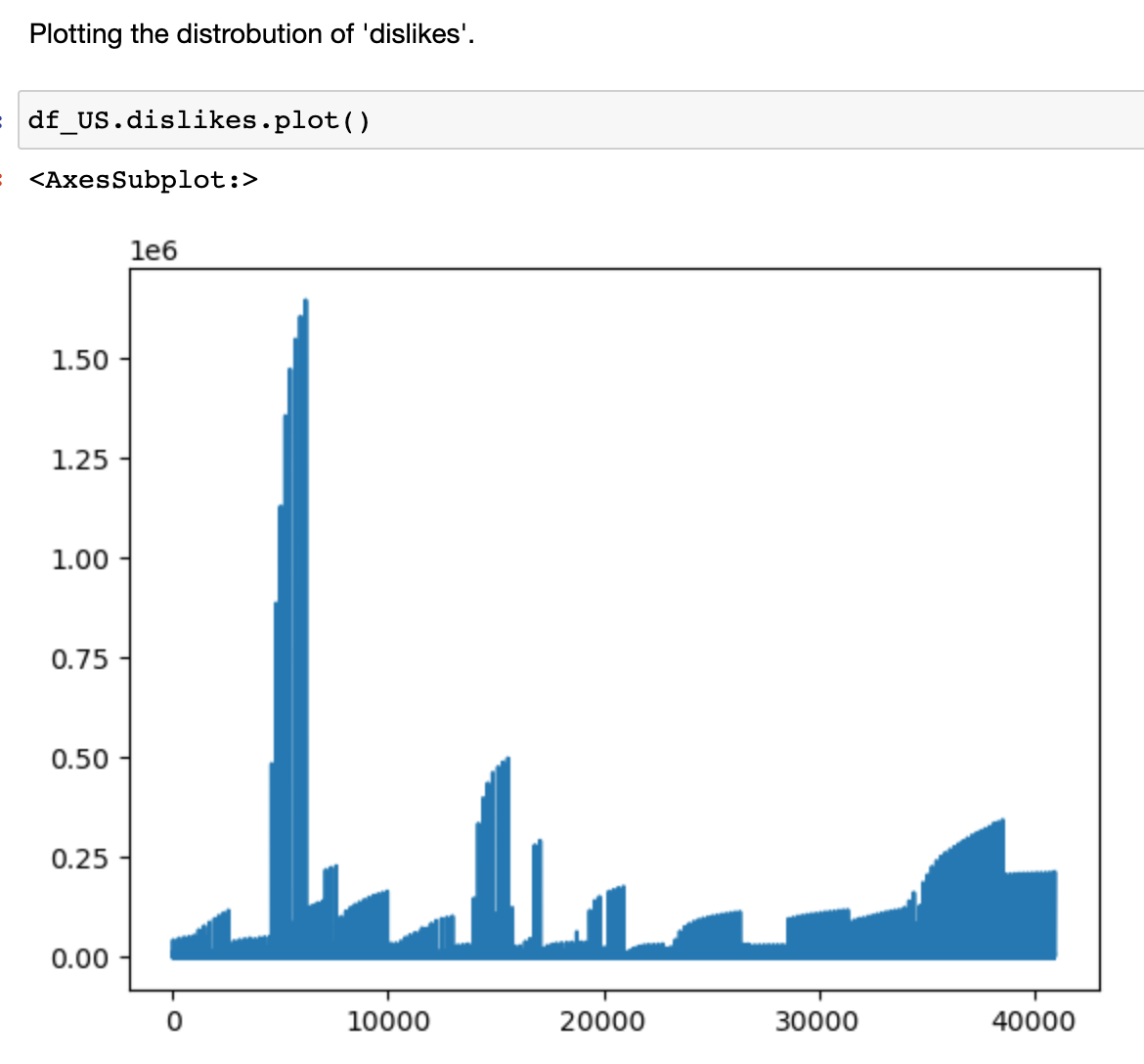
Notice that the frequency distribution appears multi-modal and right-skewed towards the 1600 hour mark. The variables appear to be non-parametric. The same pattern will be apparent in the following visualizations of ‘comment_count’, ‘views’, and ‘likes’. The multi-modality will be more pronounced. Noticeably, the fourth visualization ‘dislikes’, will take a sharp distribution direction change and be commandingly left-skewed.

Bivariate Exploration

The below visualization is a jointplot, comparing ‘views’, ‘likes’, and ‘upload_hour’. The graph shows that the amount of ‘likes’ and ‘views’, hued in four-hour increments; Trends highest towards the ‘0400’ hour. Videos uploaded towards the 0400 hour get more than double the number of views compared to the 0800 hour and almost 4x the amount of views as the 1600 hour. Also, the number of likes (on the low estimate) for the 0400 group, is double that of the 1600 group.

The following visualizations demonstrate the variables of ‘views’, ‘likes’, ‘dislikes’, and ‘comment_count’, individually paired against ‘upload_hour’. Notice that the distributions are now all left-skewed, bracketing between approximately the 0400 and 0900 hours for all the below graphs (up to the KPI visualization).

3D graphs of views, likes, and upload hour.

jointplot() plots the relationship or joint distribution of two variables while adding marginal axes that show the univariate distribution of each one separately.

Imagine the video content is a rubber ball and if you drop your rubber ball at a certain time, the ball will bounce a certain hieght.

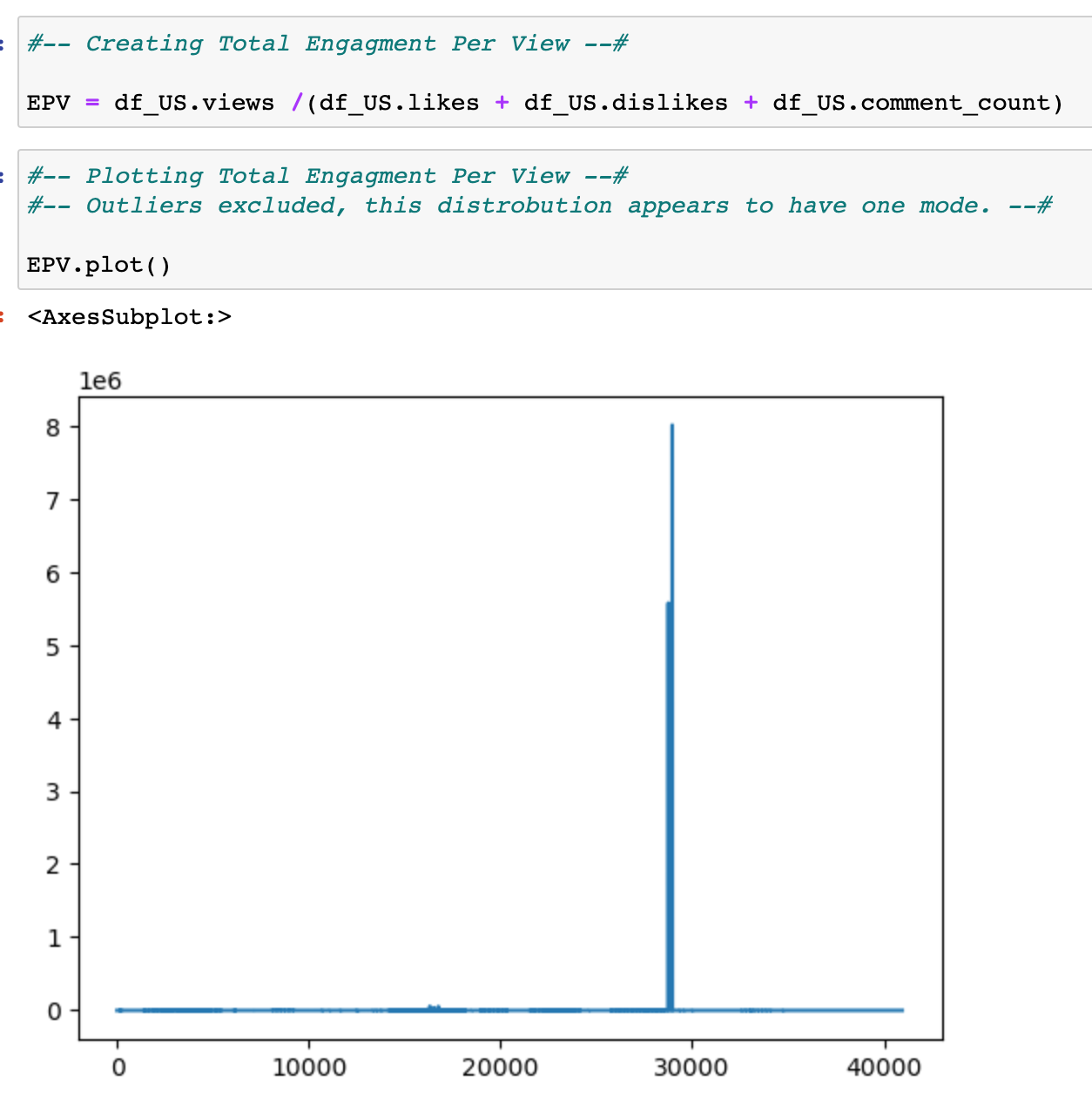
Creating the KPI for exploration.¶

Engagement Per View (EPV) = 'views' / ('likes' + 'dislikes' + 'comment_count')

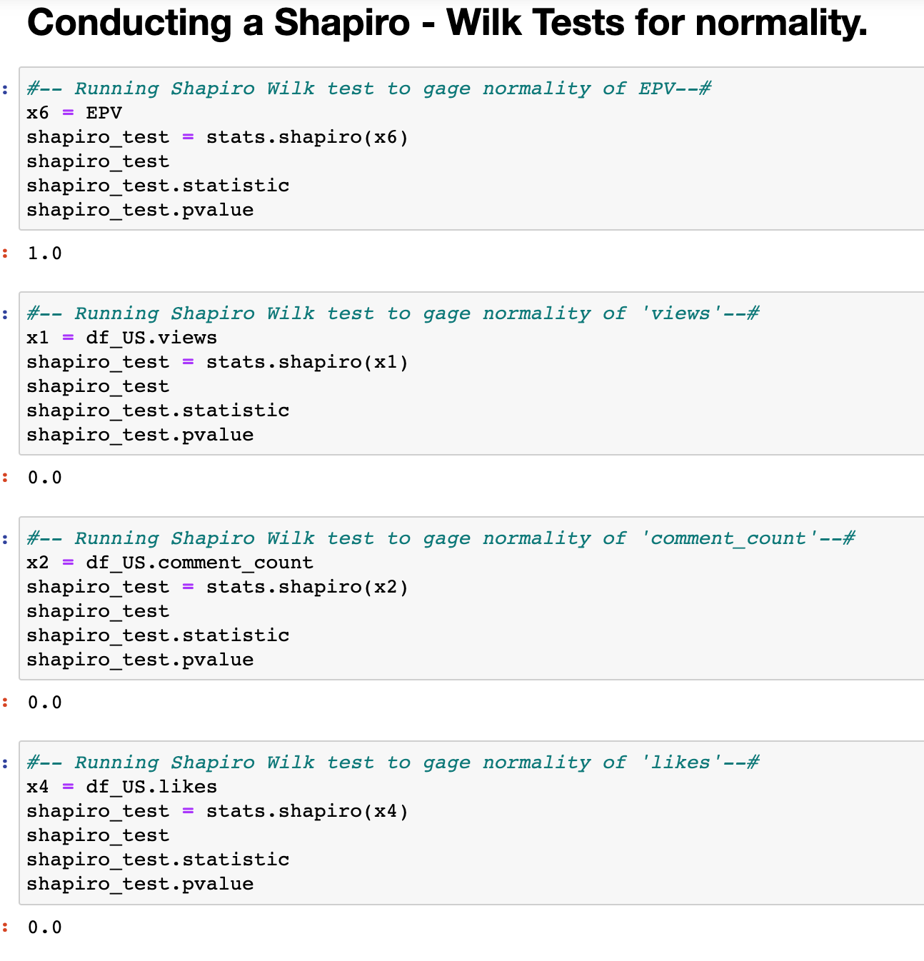
Conducting a Shapiro - Wilk Tests for normality.¶

The below Shapiro -Wilk test of EPV outputs a p-value =1; Which is greater than .05, indicating that EPV is a ‘normal’ distribution. On the other hand, the remaining variables all had p-values = 0.0, less than .05, and therefore the null hypothesis of ‘normality’ is rejected.

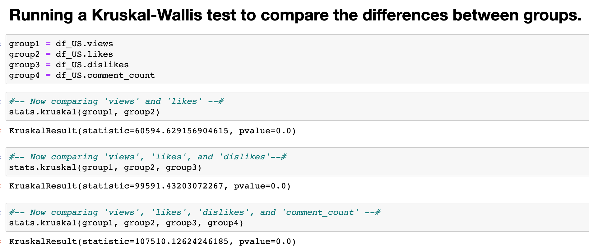
Because of the non-parametric nature of the variables, the Kruskal-Wallis test for similarity between groups is appropriate. The resulting output for all Kruskal-Wallis tests between group combinations yielded the same p-values equaling zero. Secondly, the H- statistic continued to increase as more groups were added. Ergo, rejecting the null hypothesis in support of the Alternative Hypothesis; At least two of the four populations differ.

Data Summary and Implications

The Kruskal – Wallis test answered the research question with the stated groups and the Null Hypothesis was rejected in support of the Alternative Hypothesis; none of the individual variables came from a normal distribution. Only when the variables where combined into EPV, did it test positive to being Gaussian in nature, via the Shapiro-Wilk test; All the other variables, failed to be of a normal distribution. Moreover, with the exception of ‘dislikes’, the remaining variables indicate similar multi-modal distributions. When studied individually or against ‘upload_hour’, the variables exhibit the same non-parametric behavior but skewed in the opposite direction. What is interesting is the bell-shaped distribution discovered only around the 0500 Zulu time with the EPV metric. What this research might imply is that 0500 Zulu time is the only time to receive positive Engagement Per View. Since the dataset only covered trending YouTube Videos in the United States, one recommended course of action is to compare the datasets of other countries that are available to the public at Kaggle.com. One limitation of the analysis is that only one categorical variable was explored. Therefore, one direction for future study with the dataset, is to explore the video ‘categories’ variable with the same engagement variables. Another direction for future study, would be to compare video ‘titles’ variable against the same engagement metrics, to find trending key-word phrases.

Work Cited

GATR Journal of Management and Marketing Review - researchgate.net. (n.d.). Retrieved February 9, 2023, from https://www.researchgate.net/profile/Richard-Fedorko/publication/347381995_Brand_Engagement_in_the_Light_of_Post_Content_Type_on_the_Facebook_Platform_in_the_Selected_Industry/links/6110e7a00c2bfa282a2f9401/Brand-Engagement-in-the-Light-of-Post-Content-Type-on-the-Facebook-Platform-in-the-Selected-Industry.pdf

J, M. (2019, June 3). Trending YouTube video statistics. Kaggle. Retrieved February 8, 2023, from https://www.kaggle.com/datasets/datasnaek/youtube-new?select=USvideos.csv

Pandey, Y. (n.d.). SAS vs python. LinkedIn. Retrieved February 8, 2023, from https://www.linkedin.com/pulse/sas-vs-python-yuvaraj-pandey/

Python vs. R: What's the difference? IBM. (n.d.). Retrieved February 8, 2023, from https://www.ibm.com/cloud/blog/python-vs-r

Scipy.stats.kruskal#. scipy.stats.kruskal - SciPy v1.10.0 Manual. (n.d.). Retrieved February 8, 2023, from https://docs.scipy.org/doc/scipy/reference/generated/scipy.stats.kruskal.html

Zach. (2022, March 7). Kruskal-Wallis test: Definition, formula, and example. Statology. Retrieved February 8, 2023, from https://www.statology.org/kruskal-wallis-test/

Check out other blogs on the similar topics:

When should you upload to YouTube in 2023?

STOP USING HASHTAGS 2023

Podcast Interview with ChatGTP

Forecasting with Time Series Data

Natural Language Processing on IMDB movie comments

Principal Component Analysis with Telecom Data

Market Basket Analysis for Prescription Data

Hacking the System: Optimizing Humans to Increase Page Ranking

Drug Overdose Deaths Data Mining Exploration

Random Forrest with Python

Hospital Readmission Tool Dashboard